Plot track density#
[1]:
import huracanpy

import cartopy.crs as ccrs
Basic routine#
[2]:
# Load data (example : ibtracs)
tracks = huracanpy.load(source="ibtracs")
/home/docs/checkouts/readthedocs.org/user_builds/huracanpy/envs/v1-doc/lib/python3.12/site-packages/huracanpy/_data/ibtracs.py:112: UserWarning: This offline function loads a light version of IBTrACS which is embedded within the package, based on a file produced manually by the developers.
                  It was last updated on the 15th Nov 2024, based on the IBTrACS file at that date.
                  It contains only data from 1980 up to the last year with no provisional tracks. All spur tracks were removed. Only 6-hourly time steps were kept.
  warnings.warn(
/home/docs/checkouts/readthedocs.org/user_builds/huracanpy/envs/v1-doc/lib/python3.12/site-packages/huracanpy/_data/ibtracs.py:118: UserWarning: You are loading the IBTrACS-WMO subset.                       This dataset contains the positions and intensity reported by the WMO agency responsible for each basin
                      Be aware of the fact that wind and pressure data is provided as they are in IBTrACS,                       which means in particular that wind speeds are in knots and averaged over different time periods.
                    For more information, see the IBTrACS column documentation at https://www.ncei.noaa.gov/sites/default/files/2021-07/IBTrACS_v04_column_documentation.pdf
  warnings.warn(
To plot the track density, you need two functions. The first one, huracanpy.diags.track_density.simple_global_histogram computes the track density, which is stored in a 2D xarray. The second one huracanpy.plot.density.plot_density will plot the track density. Because the track density is a xarray object, you can also use built-in xarray functions.
[3]:
# Compute track density
D = huracanpy.calc.density(tracks.lon, tracks.lat)
D  # D, the track density, is a map stored in xarray
[3]:
<xarray.DataArray (lat: 29, lon: 72)> Size: 17kB
array([[0., 0., 0., ..., 0., 2., 0.],
       [0., 0., 0., ..., 0., 0., 2.],
       [0., 0., 0., ..., 0., 1., 2.],
       ...,
       [0., 0., 0., ..., 1., 4., 4.],
       [0., 0., 0., ..., 0., 0., 1.],
       [0., 0., 0., ..., 0., 0., 0.]], shape=(29, 72))
Coordinates:
  * lon      (lon) float64 576B -177.5 -172.5 -167.5 ... 167.5 172.5 177.5
* lat (lat) float64 232B -67.5 -62.5 -57.5 -52.5 ... 57.5 62.5 67.5 72.5[4]:
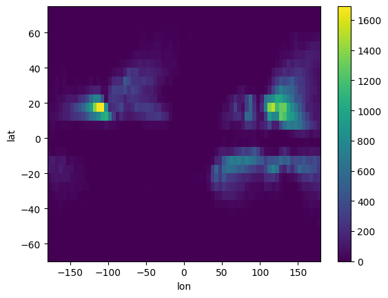
# Plotting using huracanpy function
huracanpy.plot.density(D)
[4]:
(<Figure size 640x480 with 2 Axes>, <GeoAxes: xlabel='lon', ylabel='lat'>)
[5]:
# Plotting using xarray's plot function
D.plot()
[5]:
<matplotlib.collections.QuadMesh at 0x7fe68ec6e780>
Customization#
Density computation#
For the track density computation, there are two things that can be customized :
bin_size: The size of the boxes over which the track density is computed, in degrees.N_seasonsis a normalization factor. It is useful to make the number make sense, such as “number of TC point per year in abin_size x bin_sizebox”
[6]:
# Setting a smaller bin_size
D = huracanpy.calc.density(tracks.lon, tracks.lat, bin_size=1)
D.plot()
D
[6]:
<xarray.DataArray (lat: 133, lon: 357)> Size: 380kB
array([[0., 0., 0., ..., 0., 0., 0.],
       [0., 0., 0., ..., 0., 0., 0.],
       [0., 0., 0., ..., 0., 0., 0.],
       ...,
       [0., 0., 0., ..., 0., 0., 0.],
       [0., 0., 0., ..., 0., 0., 1.],
       [0., 0., 0., ..., 0., 0., 0.]], shape=(133, 357))
Coordinates:
  * lon      (lon) float64 3kB -179.5 -178.5 -177.5 -176.5 ... 177.5 178.5 179.5
  * lat      (lat) float64 1kB -68.5 -67.5 -66.5 -63.5 ... 67.5 68.5 69.5 70.5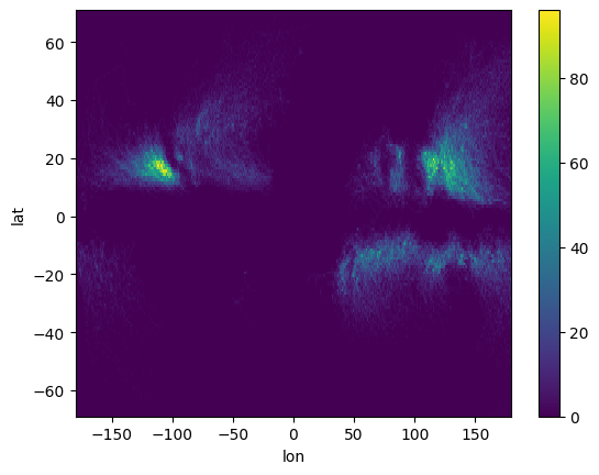
[7]:
# Setting a larger bin_size
D = huracanpy.calc.density(tracks.lon, tracks.lat, bin_size=10)
D.plot()
D
[7]:
<xarray.DataArray (lat: 15, lon: 36)> Size: 4kB
array([[0.000e+00, 0.000e+00, 0.000e+00, 0.000e+00, 0.000e+00, 1.000e+00,
        1.000e+00, 0.000e+00, 0.000e+00, 0.000e+00, 0.000e+00, 0.000e+00,
        0.000e+00, 0.000e+00, 0.000e+00, 0.000e+00, 0.000e+00, 0.000e+00,
        0.000e+00, 0.000e+00, 0.000e+00, 0.000e+00, 0.000e+00, 0.000e+00,
        0.000e+00, 0.000e+00, 0.000e+00, 0.000e+00, 0.000e+00, 0.000e+00,
        0.000e+00, 0.000e+00, 0.000e+00, 0.000e+00, 1.000e+00, 4.000e+00],
       [0.000e+00, 3.000e+00, 2.000e+00, 4.000e+00, 5.000e+00, 2.000e+00,
        2.000e+00, 0.000e+00, 0.000e+00, 0.000e+00, 0.000e+00, 0.000e+00,
        0.000e+00, 0.000e+00, 0.000e+00, 0.000e+00, 0.000e+00, 0.000e+00,
        0.000e+00, 0.000e+00, 0.000e+00, 0.000e+00, 0.000e+00, 0.000e+00,
        0.000e+00, 0.000e+00, 0.000e+00, 0.000e+00, 0.000e+00, 0.000e+00,
        0.000e+00, 0.000e+00, 0.000e+00, 0.000e+00, 3.000e+00, 9.000e+00],
       [2.000e+00, 2.100e+01, 1.800e+01, 1.100e+01, 5.000e+00, 4.000e+00,
        3.000e+00, 0.000e+00, 0.000e+00, 0.000e+00, 0.000e+00, 0.000e+00,
        0.000e+00, 0.000e+00, 0.000e+00, 0.000e+00, 0.000e+00, 0.000e+00,
        0.000e+00, 0.000e+00, 0.000e+00, 0.000e+00, 5.000e+00, 8.000e+00,
        2.100e+01, 1.000e+01, 7.000e+00, 2.000e+00, 0.000e+00, 0.000e+00,
        0.000e+00, 0.000e+00, 0.000e+00, 1.600e+01, 4.000e+01, 4.400e+01],
       [1.300e+01, 9.100e+01, 7.500e+01, 6.000e+01, 3.800e+01, 1.200e+01,
        1.600e+01, 1.000e+00, 0.000e+00, 0.000e+00, 0.000e+00, 0.000e+00,
...
        0.000e+00, 0.000e+00, 0.000e+00, 0.000e+00, 0.000e+00, 8.000e+00,
        1.100e+02, 3.370e+02, 4.280e+02, 4.930e+02, 5.540e+02, 4.080e+02],
       [0.000e+00, 0.000e+00, 0.000e+00, 8.000e+00, 3.000e+00, 0.000e+00,
        0.000e+00, 0.000e+00, 0.000e+00, 3.000e+00, 3.000e+00, 6.000e+00,
        5.800e+01, 6.400e+01, 1.040e+02, 6.400e+01, 6.500e+01, 3.100e+01,
        1.900e+01, 0.000e+00, 0.000e+00, 0.000e+00, 0.000e+00, 0.000e+00,
        0.000e+00, 0.000e+00, 0.000e+00, 0.000e+00, 0.000e+00, 3.000e+00,
        1.600e+01, 3.300e+01, 1.610e+02, 1.180e+02, 1.910e+02, 2.610e+02],
       [0.000e+00, 0.000e+00, 0.000e+00, 0.000e+00, 1.000e+00, 0.000e+00,
        0.000e+00, 0.000e+00, 0.000e+00, 0.000e+00, 0.000e+00, 0.000e+00,
        1.700e+01, 2.000e+00, 9.000e+00, 2.400e+01, 2.800e+01, 1.500e+01,
        6.000e+00, 3.000e+00, 0.000e+00, 0.000e+00, 0.000e+00, 0.000e+00,
        0.000e+00, 0.000e+00, 0.000e+00, 0.000e+00, 0.000e+00, 0.000e+00,
        0.000e+00, 1.000e+00, 1.000e+01, 2.000e+00, 4.000e+00, 9.000e+00],
       [0.000e+00, 0.000e+00, 0.000e+00, 0.000e+00, 0.000e+00, 0.000e+00,
        0.000e+00, 0.000e+00, 0.000e+00, 0.000e+00, 0.000e+00, 0.000e+00,
        0.000e+00, 0.000e+00, 0.000e+00, 0.000e+00, 0.000e+00, 1.000e+00,
        0.000e+00, 0.000e+00, 0.000e+00, 0.000e+00, 0.000e+00, 0.000e+00,
        0.000e+00, 0.000e+00, 0.000e+00, 0.000e+00, 0.000e+00, 0.000e+00,
        0.000e+00, 0.000e+00, 0.000e+00, 0.000e+00, 0.000e+00, 0.000e+00]])
Coordinates:
  * lon      (lon) float64 288B -175.0 -165.0 -155.0 ... 155.0 165.0 175.0
  * lat      (lat) float64 120B -65.0 -55.0 -45.0 -35.0 ... 45.0 55.0 65.0 75.0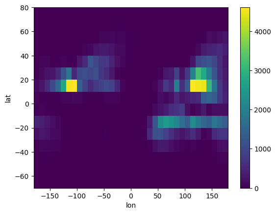
[8]:
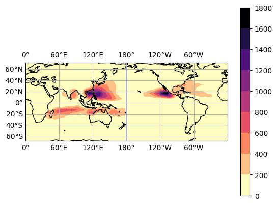
# Normalizing
## Computing the number of season in the dataset
import numpy as np
N = len(np.unique(tracks.season.values))
print(N)
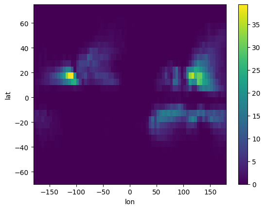
## Track density with normalization.
D = huracanpy.calc.density(tracks.lon, tracks.lat, n_seasons=N)
# In this case, now the number in D in number of TC points in each 5x5 box.
D.plot()
43
[8]:
<matplotlib.collections.QuadMesh at 0x7fe68efa7b60>
Plotting#
[9]:
# With huracanpy's function
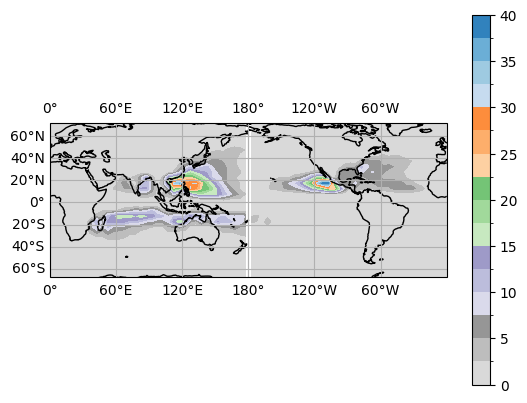
## The function is based on matplotlib's contourf, so you can use its options
huracanpy.plot.density(D, contourf_kws=dict(cmap="tab20c_r", levels=20))
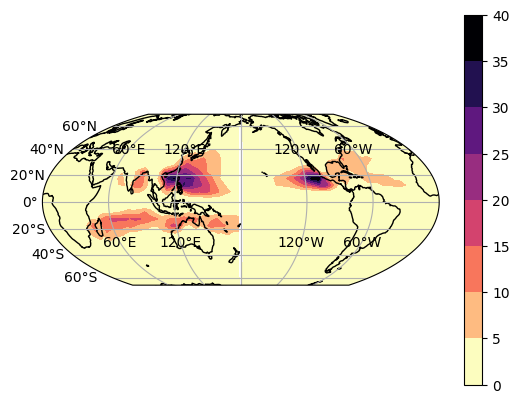
## Changing the projection with subplot_kws
huracanpy.plot.density(D, subplot_kws=dict(projection=ccrs.Mollweide(180)))
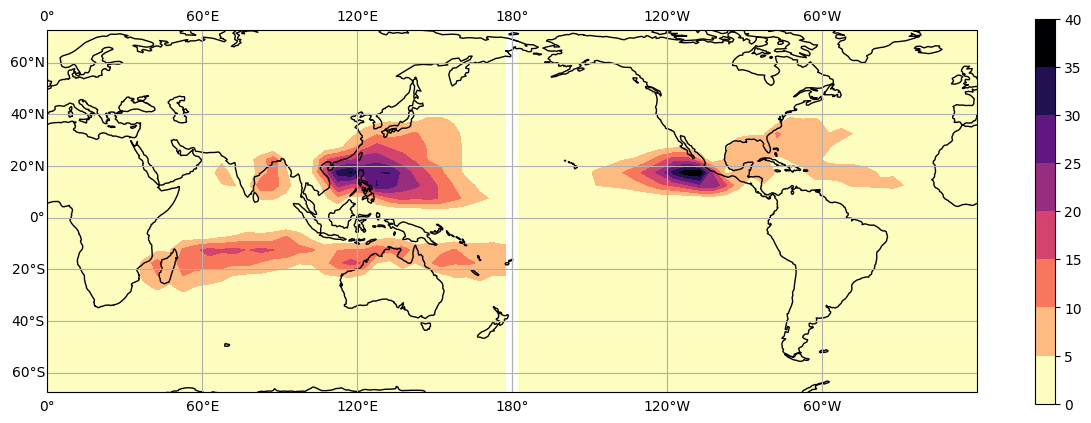
## Changing the figure's properties
huracanpy.plot.density(D, fig_kws=dict(figsize=(15, 5)))
[9]:
(<Figure size 1500x500 with 2 Axes>, <GeoAxes: xlabel='lon', ylabel='lat'>)