1. Studying a specific cyclone#

In this example, we want to study hurricane Wilma (the deepest Atlantic hurricane on record).

[1]:

import huracanpy
import matplotlib.pyplot as plt

1.2. Add category info#

You can add the Saffir-Simpson and/or the pressure category of Wilma to the tracks (for full list of available info, see huracanpy.info).

1.2.1. Add Saffir-Simpson Category#

This is stored in the saffir_simpson_category variable

[5]:

wilma = wilma.hrcn.add_saffir_simpson_category(wind_name="wind", wind_units="knots")
wilma.saffir_simpson_category

[5]:

<xarray.DataArray 'saffir_simpson_category' (record: 45)> Size: 360B
array([-1, -1, -1, -1, -1, -1,  0,  0,  0,  0,  1,  1,  2,  5,  5,  5,  5,
        5,  5,  5,  5,  5,  5,  5,  4,  4,  4,  3,  2,  2,  2,  2,  3,  3,
        4,  3,  4,  4,  3,  3,  2,  1,  0,  0,  0])
Dimensions without coordinates: record

1.2.2. Add pressure category#

[6]:

wilma = wilma.hrcn.add_pressure_category(slp_name="slp")
wilma.pressure_category

[6]:

<xarray.DataArray 'pressure_category' (record: 45)> Size: 360B
array([0, 0, 0, 0, 0, 0, 0, 0, 0, 1, 1, 1, 2, 3, 5, 5, 5, 5, 5, 5, 5, 5,
       4, 4, 4, 4, 4, 3, 3, 3, 2, 2, 2, 3, 3, 3, 3, 3, 2, 2, 1, 1, 1, 1,
       1])
Dimensions without coordinates: record
Attributes:
    units:    dimensionless

Note: Most of the accessor methods have a get_ and an add_ version. get_ returns the values of what you ask for as a DataArray, while add_ adds it directly to the dataset with a default name. In the previous case, we could have called get_pressure_category and then save it as a variable, and potentially add it to the dataset separately

[7]:

wilma.hrcn.get_pressure_category(slp_name="slp")

[7]:

<xarray.DataArray (record: 45)> Size: 360B
array([0, 0, 0, 0, 0, 0, 0, 0, 0, 1, 1, 1, 2, 3, 5, 5, 5, 5, 5, 5, 5, 5,
       4, 4, 4, 4, 4, 3, 3, 3, 2, 2, 2, 3, 3, 3, 3, 3, 2, 2, 1, 1, 1, 1,
       1])
Dimensions without coordinates: record
Attributes:
    units:    dimensionless

1.3. Plot the track and its evolution#

1.3.1. Plot the track on a map, colored by Saffir-Simpson category#

[8]:

wilma.hrcn.plot_tracks(
    intensity_var_name="saffir_simpson_category", scatter_kws={"palette": "turbo"}
)

[8]:

(<Figure size 1000x1000 with 1 Axes>, <GeoAxes: xlabel='lon', ylabel='lat'>)

../../_images/user_guide_demos_single_cyclone_15_1.png

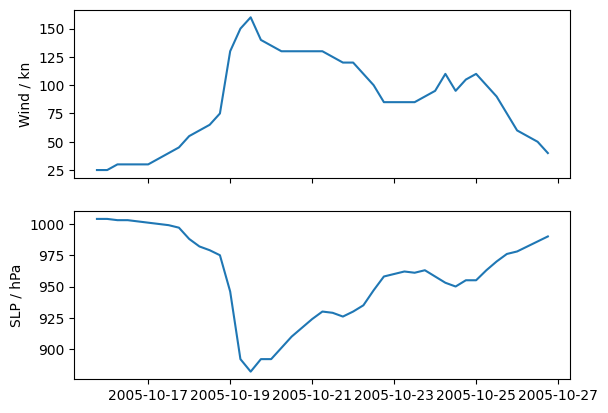
1.3.2. Plot intensity time series using matplotlib#

[9]:

fig, axs = plt.subplots(2, sharex=True)
axs[0].plot(wilma.time, wilma.wind)
axs[1].plot(wilma.time, wilma.slp)
axs[0].set_ylabel("Wind / kn")
axs[1].set_ylabel("SLP / hPa")

[9]:

Text(0, 0.5, 'SLP / hPa')

../../_images/user_guide_demos_single_cyclone_17_1.png

1.4. Calculate properties#

1.4.1. Duration#

Note duration is in hours

[10]:

wilma.hrcn.get_track_duration()

[10]:

<xarray.DataArray 'duration' (track_id: 1)> Size: 8B
array([264.])
Coordinates:
  * track_id  (track_id) object 8B '2005289N18282'
Attributes: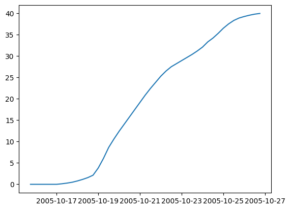
    units:    hours

1.4.2. ACE#

Accumulated cyclone energy (ACE) is a commonly used measure of cyclone activity that combines the energy and duration of cyclones.

1.4.2.1. Compute ACE for each point#

[11]:

wilma = wilma.hrcn.add_ace(wind_units="knots")
wilma.ace

[11]:

<xarray.DataArray 'ace' (record: 45)> Size: 360B
array([0.    , 0.    , 0.    , 0.    , 0.    , 0.    , 0.1225, 0.16  ,
       0.2025, 0.3025, 0.36  , 0.4225, 0.5625, 1.69  , 2.25  , 2.56  ,
       1.96  , 1.8225, 1.69  , 1.69  , 1.69  , 1.69  , 1.69  , 1.5625,
       1.44  , 1.44  , 1.21  , 1.    , 0.7225, 0.7225, 0.7225, 0.7225,
       0.81  , 0.9025, 1.21  , 0.9025, 1.1025, 1.21  , 1.    , 0.81  ,
       0.5625, 0.36  , 0.3025, 0.25  , 0.16  ])
Dimensions without coordinates: record
Attributes:
    units:    knot ** 2

1.4.2.2. Plot cumulated ACE#

[12]:

plt.plot(wilma.time, wilma.ace.cumsum())

[12]:

[<matplotlib.lines.Line2D at 0x7b938f2b6bd0>]

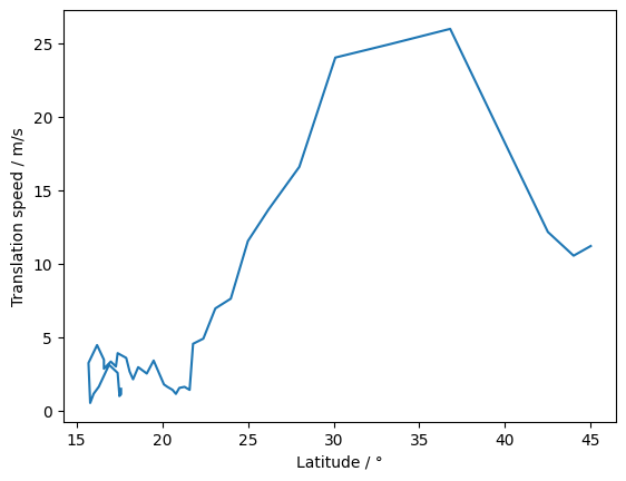
../../_images/user_guide_demos_single_cyclone_24_1.png

1.4.3. Translation speed#

1.4.3.1. Compute translation speed#

[13]:

wilma = wilma.hrcn.add_translation_speed()

1.4.3.2. Plot translation speed against latitude#

[14]:

plt.plot(wilma.lat, wilma.translation_speed)
plt.xlabel("Latitude / °")
plt.ylabel("Translation speed / m/s")

[14]:

Text(0, 0.5, 'Translation speed / m/s')

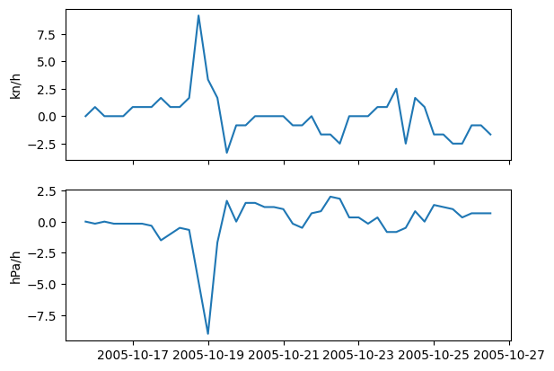
../../_images/user_guide_demos_single_cyclone_28_1.png

1.4.4. Intensification rate#

1.4.4.1. Add intensification rate in wind and pressure#

NB: The rates will be in unit/s, where unit is the unit of the variable.

[15]:

wilma = wilma.hrcn.add_rate(var_name="wind")
wilma = wilma.hrcn.add_rate(var_name="slp")

1.4.4.2. Plot intensity time series#

[16]:

fig, axs = plt.subplots(2, sharex=True)
# Convert to kn/h and hPa/h
axs[0].plot(wilma.time, wilma.rate_wind * 3600)
axs[1].plot(wilma.time, wilma.rate_slp * 3600)
axs[0].set_ylabel("kn/h")
axs[1].set_ylabel("hPa/h")

[16]:

Text(0, 0.5, 'hPa/h')

../../_images/user_guide_demos_single_cyclone_32_1.png