3. Comparing two datasets

In this part, we compare the set of 1996 tracks (used in the previous example) to IBTrACS which we use as reference. To start with, note that for all that was shown in the previous examples, you can superimpose several sets and therefore compare several sources/models/trackers/etc. Below we show specific functions for matching tracks and computing detection scores.

import huracanpy
import matplotlib.pyplot as plt

3.1. Load tracks

3.1.1. Load IBTrACS and subset the 1996 tracks with xarray’s where method

ib = huracanpy.load(source="ibtracs")
ib_1996 = ib.where(ib.time.dt.year == 1996, drop=True)
ib_1996

/home/docs/checkouts/readthedocs.org/user_builds/huracanpy/envs/stable/lib/python3.12/site-packages/huracanpy/_data/ibtracs.py:119: UserWarning: This offline function loads a light version of IBTrACS which is embedded within the package, based on a file produced manually by the developers.
 It was last updated on the 15th Nov 2024, based on the IBTrACS file at that date.
 It contains only data from 1980 up to the last year with no provisional tracks. All spur tracks were removed. Only 6-hourly time steps were kept.
  warnings.warn(
/home/docs/checkouts/readthedocs.org/user_builds/huracanpy/envs/stable/lib/python3.12/site-packages/huracanpy/_data/ibtracs.py:128: UserWarning: You are loading the IBTrACS-WMO subset. This dataset contains the positions and intensity reported by the WMO agency responsible for each basin
 Be aware of the fact that wind and pressure data is provided as they are in IBTrACS, which means in particular that wind speeds are in knots and averaged over different time periods.
 For more information, see the IBTrACS column documentation at https://www.ncei.noaa.gov/sites/default/files/2021-07/IBTrACS_v04_column_documentation.pdf
  warnings.warn(

<xarray.Dataset> Size: 276kB
Dimensions:   (record: 4313)
Dimensions without coordinates: record
Data variables:
    track_id  (record) object 35kB '1995357N07139' ... '1996365S15137'
    season    (record) float64 35kB 1.995e+03 1.995e+03 ... 1.997e+03 1.997e+03
    basin     (record) object 35kB 'WP' 'WP' 'WP' 'WP' ... 'SP' 'SI' 'SI' 'SI'
    time      (record) datetime64[s] 35kB 1996-01-01 ... 1996-12-31T18:00:00
    lon       (record) float64 35kB 153.5 157.0 159.0 ... 134.6 134.1 133.8
    lat       (record) float64 35kB 26.0 27.0 27.5 28.0 ... -13.6 -13.2 -12.8
    wind      (record) float64 35kB nan nan nan nan nan ... nan nan nan nan nan
    slp       (record) float64 35kB 1.008e+03 1.006e+03 1.006e+03 ... nan nan

xarray.Dataset

• Dimensions:
  • record: 4313
• Data variables: (8)
  • track_id
    (record)
    object
    '1995357N07139' ... '1996365S15137'

    cf_role :

    trajectory_id

    array(['1995357N07139', '1995357N07139', '1995357N07139', ...,
           '1996365S15137', '1996365S15137', '1996365S15137'],
          shape=(4313,), dtype=object)

  • season
    (record)
    float64
    1.995e+03 1.995e+03 ... 1.997e+03

    array([1995., 1995., 1995., ..., 1997., 1997., 1997.], shape=(4313,))

  • basin
    (record)
    object
    'WP' 'WP' 'WP' ... 'SI' 'SI' 'SI'

    array(['WP', 'WP', 'WP', ..., 'SI', 'SI', 'SI'],
          shape=(4313,), dtype=object)

  • time
    (record)
    datetime64[s]
    1996-01-01 ... 1996-12-31T18:00:00

    array(['1996-01-01T00:00:00', '1996-01-01T06:00:00',
           '1996-01-01T12:00:00', ..., '1996-12-31T06:00:00',
           '1996-12-31T12:00:00', '1996-12-31T18:00:00'],
          shape=(4313,), dtype='datetime64[s]')

  • lon
    (record)
    float64
    153.5 157.0 159.0 ... 134.1 133.8

    array([153.5, 157. , 159. , ..., 134.6, 134.1, 133.8], shape=(4313,))

  • lat
    (record)
    float64
    26.0 27.0 27.5 ... -13.2 -12.8

    array([ 26. ,  27. ,  27.5, ..., -13.6, -13.2, -12.8], shape=(4313,))

  • wind
    (record)
    float64
    nan nan nan nan ... nan nan nan nan

    array([nan, nan, nan, ..., nan, nan, nan], shape=(4313,))

  • slp
    (record)
    float64
    1.008e+03 1.006e+03 ... nan nan

    array([1008., 1006., 1006., ...,   nan,   nan,   nan], shape=(4313,))

3.1.2. Load ERA5 year of tracks

era5 = huracanpy.load(huracanpy.example_year_file)

3.2. Superimposing several sets on one plot

To start with, note that for all that was shown above, you can superimpose several sets and therefore compare several sources/models/trackers/etc. Here we only show one example.

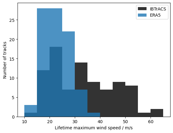
3.2.1. Compute lifetime maximum intensity (LMI) for both sets

lmi_wind_ib = ib_1996.wind.groupby(ib_1996.track_id).max()
# Convert kn to m/s
lmi_wind_ib = lmi_wind_ib / 1.94
lmi_wind_era5 = era5.wind10.groupby(era5.track_id).max()

3.2.2. Plot both histograms

bins = range(10, 65 + 1, 5)
lmi_wind_ib.plot.hist(bins=bins, color="k", label="IBTrACS", alpha=0.8)
lmi_wind_era5.plot.hist(bins=bins, label="ERA5", alpha=0.8)
plt.legend()
plt.xlabel("Lifetime maximum wind speed / m/s")
plt.ylabel("Number of tracks")

Text(0, 0.5, 'Number of tracks')

3.3. Matching tracks

Use huracanpy.assess.match to find matching tracks. The results is a pandas.DataFrame where each row is a pair of tracks that matched, with both ids, the number of time steps and the mean distance between the tracks over their matching period.

matches = huracanpy.assess.match([era5, ib_1996], names=["ERA5", "IBTrACS"])
matches

	id_ERA5	id_IBTrACS	temp	dist
0	1207.0	1996002S15133	27	48.531963
1	1208.0	1996001S08075	39	39.697687
2	1209.0	1996007S10100	13	80.979701
3	1210.0	1996015S18182	13	104.460676
4	1213.0	1996021S16152	11	70.118845
...	...	...	...	...
72	1291.0	1996353N05151	26	64.419466
73	1292.0	1996357S10136	30	96.003139
74	1293.0	1996356N08110	13	98.513440
75	1294.0	1996354S05170	32	86.234183
76	1295.0	1996365S15137	1	134.400469

77 rows × 4 columns

3.4. Computing scores

3.4.1. Probability of detection (POD)

Proportion of observed tracks that are found in ERA5.

huracanpy.assess.pod(matches, ref=ib_1996, ref_name="IBTrACS")

0.635593220338983

3.4.2. False alarm rate (FAR)

Proportion of detected tracks that were not observed

huracanpy.assess.far(matches, detected=era5, detected_name="ERA5")

0.1460674157303371

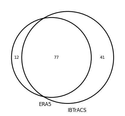
3.5. Venn diagrams

Venn diagrams are a convenient way to show the overlap between two datasets.

huracanpy.plot.venn([era5, ib_1996], matches, labels=["ERA5", "IBTrACS"])