2. Studying a set of tracks#
[1]:
import huracanpy
import numpy as np
import seaborn as sns
2.1. Load tracks#
Here we show an example with a CSV file that is embedded within HuracanPy. HuracanPy supports many track file formats, see huracanpy.load guide for more details.
Load the ERA5 1996 TC tracks with huracanpy.load. These are tracks detected by TempestExtremes in ERA5 for the year 1996 and are embedded within HuracanPy as an example. Here the file extension is ‘.csv’, the function will automatically recognise how to open it.
The tracks are loaded as an xarray.Dataset, with one dimension “record” corresponding to each point. Variables indicate position in space and time, as well as additional attributes such as maximum wind speed and minimum slp.
[2]:
file = huracanpy.example_year_file
print(file.split("/")[-1])

tracks = huracanpy.load(file)
tracks
ERA5_1996_UZ.csv
[2]:
<xarray.Dataset> Size: 236kB
Dimensions:   (record: 2274)
Dimensions without coordinates: record
Data variables: (12/13)
    track_id  (record) float64 18kB 1.207e+03 1.207e+03 ... 1.294e+03 1.295e+03
    year      (record) float64 18kB 1.996e+03 1.996e+03 ... 1.996e+03 1.996e+03
    month     (record) float64 18kB 1.0 1.0 1.0 1.0 1.0 ... 12.0 12.0 12.0 12.0
    day       (record) float64 18kB 3.0 3.0 3.0 3.0 4.0 ... 31.0 31.0 31.0 31.0
    hour      (record) float64 18kB 0.0 6.0 12.0 18.0 0.0 ... 6.0 12.0 18.0 18.0
    i         (record) float64 18kB 549.0 550.0 550.0 ... 737.0 754.0 540.0
    ...        ...
    lon       (record) float64 18kB 137.2 137.5 137.5 ... 184.2 188.5 135.0
    lat       (record) float64 18kB -15.5 -15.25 -14.75 ... -47.0 -48.5 -12.5
    slp       (record) float64 18kB 1.006e+05 1.002e+05 ... 9.848e+04 1.005e+05
    zs        (record) float64 18kB 52.12 13.98 32.58 ... -124.6 -128.8 44.54
    wind10    (record) float64 18kB 9.561 11.16 11.03 ... 21.39 21.11 11.58
time (record) datetime64[s] 18kB 1996-01-03 ... 1996-12-31T18:00:002.2. Adding info to the tracks#
HuracanPy has several function to add useful information to the tracks (for full list, see huracanpy.info). Here for example we add basin and Saffir-Simpson hurrican scale category information.]
2.2.1. Add basin#
[3]:
tracks = tracks.hrcn.add_basin()
tracks.basin
[3]:
<xarray.DataArray 'basin' (record: 2274)> Size: 36kB
array(['AUS', 'AUS', 'AUS', ..., 'SP', 'SP', 'AUS'],
      shape=(2274,), dtype='<U4')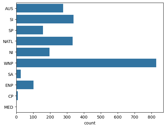
Dimensions without coordinates: record2.2.1.1. Show distribution of TC points among basins#
(calling seaborn function, works better with categorical labels)
[4]:
sns.countplot(tracks.basin)
[4]:
<Axes: xlabel='count'>
2.2.2. Add Saffir-Simpson and pressure-based categories#
Note: in ERA5 data, wind is stored in wind10 in m/s
[5]:
tracks = tracks.hrcn.add_saffir_simpson_category(wind_name="wind10", wind_units="m s-1")
tracks = tracks.hrcn.add_pressure_category(slp_name="slp", slp_units="Pa")
tracks[["saffir_simpson_category", "pressure_category"]]
[5]:
<xarray.Dataset> Size: 36kB
Dimensions:                  (record: 2274)
Dimensions without coordinates: record
Data variables:
    saffir_simpson_category  (record) int64 18kB -1 -1 -1 -1 -1 ... 0 0 0 0 -1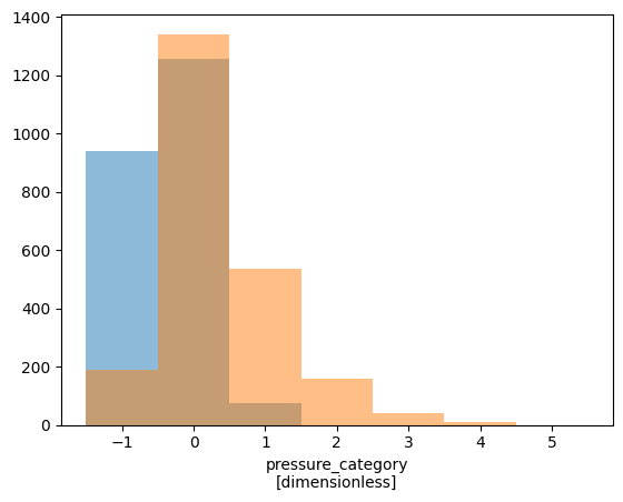
pressure_category (record) int64 18kB -1 0 0 0 0 0 0 ... 1 1 1 1 1 -12.2.2.1. Show distribution of TC points among categories#
(using xarray’s built-in function)
[6]:
bins = np.arange(-1.5, 5.5 + 1)
tracks.saffir_simpson_category.plot.hist(bins=bins, alpha=0.5)
tracks.pressure_category.plot.hist(bins=bins, alpha=0.5)
[6]:
(array([ 190., 1342.,  534.,  157.,   41.,   10.,    0.]),
 array([-1.5, -0.5,  0.5,  1.5,  2.5,  3.5,  4.5,  5.5]),
 <BarContainer object of 7 artists>)
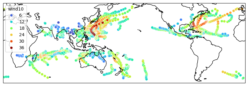
2.3. Plotting#
HuracanPy embeds basic plotting functions, which are mainly meant for having a preliminary look at your data. In particular here we show how to plot the track points themselves, and track density. The example gallery displays nice plots made from HuracanPy and the associated scripts. ### Plotting the tracks Plot ERA5 tracks colored by wind intensity
[7]:
tracks.hrcn.plot_tracks(intensity_var_name="wind10")
[7]:
(<Figure size 1000x1000 with 1 Axes>, <GeoAxes: xlabel='lon', ylabel='lat'>)
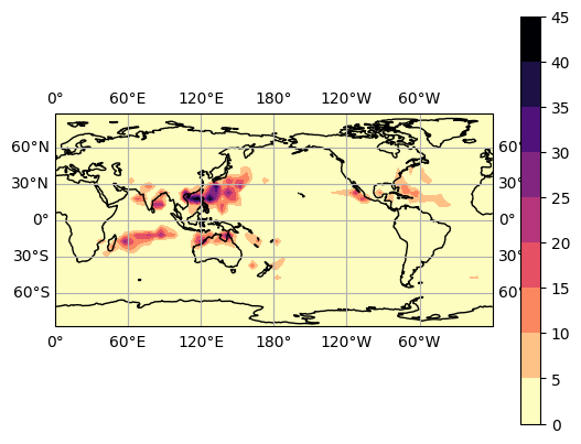
2.3.1. Plotting track density#
You can plot the track density directly with plot_density, which is based on a simple 2D histogram of TC points
[8]:
tracks.hrcn.plot_density()
/home/docs/checkouts/readthedocs.org/user_builds/huracanpy/envs/v1.4.0/lib/python3.12/site-packages/huracanpy/calc/_density.py:88: UserWarning: By default density does not take into account the spherical geometry ofthe Earth. Set spherical=True to account for this
  warnings.warn(
[8]:
(<Figure size 640x480 with 2 Axes>, <GeoAxes: xlabel='lon', ylabel='lat'>)
You can also get the underlying density matrix with get_density and then use it to make you own plots in your favourite way
[9]:
tracks.hrcn.get_density()
/home/docs/checkouts/readthedocs.org/user_builds/huracanpy/envs/v1.4.0/lib/python3.12/site-packages/huracanpy/calc/_density.py:88: UserWarning: By default density does not take into account the spherical geometry ofthe Earth. Set spherical=True to account for this
  warnings.warn(
[9]:
<xarray.DataArray (lat: 36, lon: 72)> Size: 21kB
array([[0., 0., 0., ..., 0., 0., 0.],
       [0., 0., 0., ..., 0., 0., 0.],
       [0., 0., 0., ..., 0., 0., 0.],
       ...,
       [0., 0., 0., ..., 0., 0., 0.],
       [0., 0., 0., ..., 0., 0., 0.],
       [0., 0., 0., ..., 0., 0., 0.]], shape=(36, 72))
Coordinates:
  * lat      (lat) float64 288B -87.5 -82.5 -77.5 -72.5 ... 72.5 77.5 82.5 87.5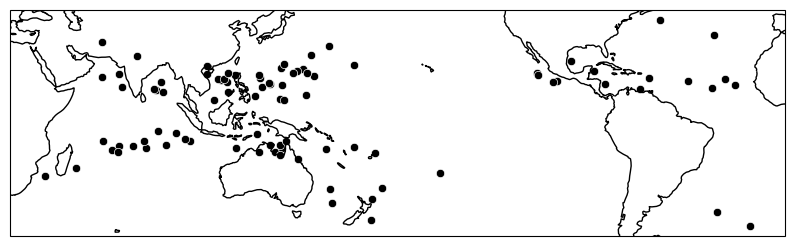
* lon (lon) float64 576B 2.5 7.5 12.5 17.5 ... 342.5 347.5 352.5 357.52.3.2. Plotting genesis points#
get_gen_vals allows you to subset only the genesis points in an efficient way
[10]:
gen_points = tracks.hrcn.get_gen_vals()
gen_points
[10]:
<xarray.Dataset> Size: 12kB
Dimensions:                  (track_id: 89)
Coordinates:
  * track_id                 (track_id) float64 712B 1.207e+03 ... 1.295e+03
Data variables: (12/15)
    year                     (track_id) float64 712B 1.996e+03 ... 1.996e+03
    month                    (track_id) float64 712B 1.0 1.0 1.0 ... 12.0 12.0
    day                      (track_id) float64 712B 3.0 5.0 6.0 ... 24.0 31.0
    hour                     (track_id) float64 712B 0.0 6.0 12.0 ... 0.0 18.0
    i                        (track_id) float64 712B 549.0 282.0 ... 636.0 540.0
    j                        (track_id) float64 712B 422.0 412.0 ... 416.0 410.0
    ...                       ...
    zs                       (track_id) float64 712B 52.12 64.94 ... 1.665 44.54
    wind10                   (track_id) float64 712B 9.561 10.54 ... 13.38 11.58
    time                     (track_id) datetime64[s] 712B 1996-01-03 ... 199...
    basin                    (track_id) <U4 1kB 'AUS' 'SI' 'AUS' ... 'AUS' 'AUS'
    saffir_simpson_category  (track_id) int64 712B -1 -1 -1 -1 ... -1 -1 -1 -1
pressure_category (track_id) int64 712B -1 -1 -1 0 -1 ... 0 0 -1 0 -1If you use plot_tracks on these, you can display only the genesis points.
[11]:
gen_points.hrcn.plot_tracks()
/home/docs/checkouts/readthedocs.org/user_builds/huracanpy/envs/v1.4.0/lib/python3.12/site-packages/huracanpy/plot/_tracks.py:56: UserWarning: Ignoring `palette` because no `hue` variable has been assigned.
  sns.scatterplot(
[11]:
(<Figure size 1000x1000 with 1 Axes>, <GeoAxes: xlabel='lon', ylabel='lat'>)
2.4. Compute statistics#
2.4.1. Number of cyclones#
Count number of unique track ids
[12]:
tracks.track_id.hrcn.nunique()
[12]:
89
2.4.2. Cyclone duration & TC days#
Get the duration for each track. The result is an xarray.Dataset with “track_id” as a coordinate
[13]:
TC_duration = tracks.hrcn.get_track_duration()
TC_duration
[13]:
<xarray.DataArray 'duration' (track_id: 89)> Size: 712B
array([162., 312.,  90., 126., 102., 126.,  96., 276.,  60.,  78., 252.,
       210., 174., 150.,  78., 180.,  66., 144., 186., 258.,  96.,  90.,
       246., 114., 114.,  84.,  72., 120., 276., 114.,  96.,  96.,  66.,
       258., 222., 312.,  78.,  72., 120., 150., 234., 324., 150.,  72.,
       354.,  54.,  96.,  90.,  96.,  90.,  90.,  84., 396., 342.,  66.,
       360., 120., 108., 114., 192., 144.,  84., 276., 198., 204., 240.,
       228., 144.,  78.,  60., 144., 330.,  66., 144., 210., 126., 294.,
        60., 204., 222.,  60., 198., 168., 144., 156., 216.,  90., 186.,
         0.])
Coordinates:
  * track_id  (track_id) float64 712B 1.207e+03 1.208e+03 ... 1.295e+03
Attributes:
units: hoursCompute the total number of TC days. Sum all the durations (and divide by 24 because durations are in hours)
[14]:
TC_duration.sum() / 24
[14]:
<xarray.DataArray 'duration' ()> Size: 8B
array(584.5)
Attributes:
units: hours2.4.3. Cyclone Intensity#
There are two ways to obtain the lifetime maximum intensity (LMI) of each tracks
Use
get_apex_vals, which returns the subset of points only at specified LMI
[15]:
lmi_points = tracks.hrcn.get_apex_vals(var_name="wind10")
lmi_points
[15]:
<xarray.Dataset> Size: 12kB
Dimensions:                  (track_id: 89)
Coordinates:
  * track_id                 (track_id) float64 712B 1.207e+03 ... 1.295e+03
Data variables: (12/15)
    year                     (track_id) float64 712B 1.996e+03 ... 1.996e+03
    month                    (track_id) float64 712B 1.0 1.0 1.0 ... 12.0 12.0
    day                      (track_id) float64 712B 6.0 10.0 10.0 ... 28.0 31.0
    hour                     (track_id) float64 712B 0.0 12.0 0.0 ... 18.0 18.0
    i                        (track_id) float64 712B 567.0 205.0 ... 687.0 540.0
    j                        (track_id) float64 712B 427.0 434.0 ... 451.0 410.0
    ...                       ...
    zs                       (track_id) float64 712B -107.4 -134.1 ... 44.54
    wind10                   (track_id) float64 712B 19.52 26.59 ... 22.33 11.58
    time                     (track_id) datetime64[s] 712B 1996-01-06 ... 199...
    basin                    (track_id) <U4 1kB 'AUS' 'SI' 'SI' ... 'SP' 'AUS'
    saffir_simpson_category  (track_id) int64 712B 0 0 0 0 0 0 ... -1 0 0 0 0 -1
pressure_category (track_id) int64 712B 1 1 0 0 0 1 ... 0 1 1 0 1 -1Compute lifetime maximum intensity per track with xarray’s
groupby
[16]:
lmi_wind = tracks.wind10.groupby(tracks.track_id).max()
lmi_wind
[16]:
<xarray.DataArray 'wind10' (track_id: 89)> Size: 712B
array([19.52451, 26.59268, 17.80909, 18.41431, 18.83423, 18.77285,
       13.04252, 22.20843, 16.17976, 17.28381, 24.70252, 26.17307,
       23.33051, 20.3704 , 20.35412, 27.6403 , 23.506  , 29.57074,
       26.85967, 28.38823, 20.47431, 15.20365, 31.37127, 20.17752,
       21.74682, 20.17922, 20.41931, 23.31932, 22.55483, 16.30926,
       21.4158 , 24.05482, 16.89222, 22.89363, 29.23333, 21.58997,
       17.58261, 21.79618, 24.55191, 29.73219, 30.8955 , 23.70912,
       20.9533 , 16.77547, 26.01644, 17.29322, 18.71597, 15.63176,
       18.66206, 23.09372, 27.94086, 20.65676, 29.73094, 27.72158,
       19.62944, 34.28312, 16.19071, 14.36055, 28.84449, 30.7681 ,
       20.81133, 15.41807, 33.45812, 27.63117, 19.58178, 31.23918,
       26.30785, 26.97909, 21.70943, 17.36107, 19.78419, 30.04986,
       19.48046, 25.52096, 20.81055, 15.8441 , 26.90078, 19.07706,
       36.74792, 17.85815, 26.09754, 18.91639, 27.87503, 15.08413,
       26.1869 , 25.00324, 22.20926, 22.3301 , 11.57796])
Coordinates:
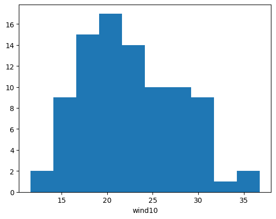
* track_id (track_id) float64 712B 1.207e+03 1.208e+03 ... 1.295e+03You can then plot the LMI distribution using xarray’s built-in plot function.
[17]:
lmi_wind.plot.hist()
[17]:
(array([ 2.,  9., 15., 17., 14., 10., 10.,  9.,  1.,  2.]),
 array([11.57796 , 14.094956, 16.611952, 19.128948, 21.645944, 24.16294 ,
        26.679936, 29.196932, 31.713928, 34.230924, 36.74792 ]),
 <BarContainer object of 10 artists>)
2.4.4. ACE#
Accumulated cyclone energy (ACE) is a commonly used measure of cyclone activity that combines the energy and duration of cyclones.
2.4.4.1. Compute ACE for each individual track point#
[18]:
tracks = tracks.hrcn.add_ace(wind_name="wind10", wind_units="m s-1")
tracks.ace
[18]:
<xarray.DataArray 'ace' (record: 2274)> Size: 18kB
array([0.        , 0.        , 0.        , ..., 0.17286087, 0.16846039,
       0.        ], shape=(2274,))
Dimensions without coordinates: record
Attributes:
units: knot ** 22.4.4.2. Compute total ACE#
[19]:
tracks.ace.sum()
[19]:
<xarray.DataArray 'ace' ()> Size: 8B
array(210.18231953)
Attributes:
units: knot ** 22.5. Compositing lifecycle#
Add time from apex variable to be able to superimpose all the tracks centered on apex. Here we use minimum pressure as the apex point
2.5.1. Add time from minimum pressure#
[20]:
tracks = tracks.hrcn.add_time_from_apex(intensity_var_name="slp", stat="min")
tracks.time_from_apex
[20]:
<xarray.DataArray 'time_from_apex' (record: 2274)> Size: 18kB
array([-237600, -216000, -194400, ...,  259200,  280800,       0],
      shape=(2274,), dtype='timedelta64[s]')
Dimensions without coordinates: record[21]:
tracks.time_from_apex / np.timedelta64(1, "h")
[21]:
<xarray.DataArray 'time_from_apex' (record: 2274)> Size: 18kB
array([-66., -60., -54., ...,  72.,  78.,   0.], shape=(2274,))
Dimensions without coordinates: record
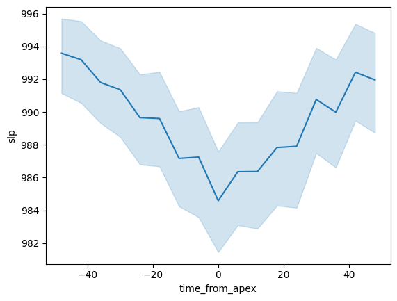
2.5.2. Plot composite SLP lifecycle#
[22]:
# Convert time_from_apex to hours
tracks["time_from_apex"] = tracks.time_from_apex / np.timedelta64(1, "h")

# Use xarray's where to mask points too far away from apex (48 hours away)
tracks_close_to_apex = tracks.where(np.abs(tracks.time_from_apex) <= 48, drop=True)

# Seaborn lineplot allows for drawing composites with uncertainty range
# x-axis is time from apex
# y-axis is slp, converted to hPa
sns.lineplot(x=tracks_close_to_apex.time_from_apex, y=tracks_close_to_apex.slp / 100)
[22]:
<Axes: xlabel='time_from_apex', ylabel='slp'>