Track density#
In this example, we show how to plot density maps (track density, genesis density, lysis density, whichever) with HuracanPy, and how to customize them.
[1]:
import huracanpy

import cartopy.crs as ccrs
[2]:
# Load data (example : ibtracs)
tracks = huracanpy.load(source="ibtracs")
/home/docs/checkouts/readthedocs.org/user_builds/huracanpy/envs/stable/lib/python3.12/site-packages/huracanpy/_data/ibtracs.py:119: UserWarning: This offline function loads a light version of IBTrACS which is embedded within the package, based on a file produced manually by the developers.
 It was last updated on the 15th Nov 2024, based on the IBTrACS file at that date.
 It contains only data from 1980 up to the last year with no provisional tracks. All spur tracks were removed. Only 6-hourly time steps were kept.
  warnings.warn(
/home/docs/checkouts/readthedocs.org/user_builds/huracanpy/envs/stable/lib/python3.12/site-packages/huracanpy/_data/ibtracs.py:128: UserWarning: You are loading the IBTrACS-WMO subset. This dataset contains the positions and intensity reported by the WMO agency responsible for each basin
 Be aware of the fact that wind and pressure data is provided as they are in IBTrACS, which means in particular that wind speeds are in knots and averaged over different time periods.
 For more information, see the IBTrACS column documentation at https://www.ncei.noaa.gov/sites/default/files/2021-07/IBTrACS_v04_column_documentation.pdf
  warnings.warn(
Basic routine#
After you loaded the data, plotting density maps is done in two very simple steps:
Computing the density;
Plotting it!
It can even be done in only one line with the accessor function.
[3]:
## Density plot from accessor: Most direct
tracks.hrcn.plot_density()
/home/docs/checkouts/readthedocs.org/user_builds/huracanpy/envs/stable/lib/python3.12/site-packages/huracanpy/calc/_density.py:88: UserWarning: By default density does not take into account the spherical geometry ofthe Earth. Set spherical=True to account for this
  warnings.warn(
[3]:
(<Figure size 640x480 with 2 Axes>, <GeoAxes: xlabel='lon', ylabel='lat'>)

[4]:
## Routine with function calls
# 1. Compute track density
D = huracanpy.calc.density(tracks.lon, tracks.lat)
# D, the track density, is a 2D map stored in xarray

# 2. Plot the track density
huracanpy.plot.density(D)
# (NB: because D is an xarray object, you can also use D.plot() directly)
/home/docs/checkouts/readthedocs.org/user_builds/huracanpy/envs/stable/lib/python3.12/site-packages/huracanpy/calc/_density.py:88: UserWarning: By default density does not take into account the spherical geometry ofthe Earth. Set spherical=True to account for this
  warnings.warn(
[4]:
(<Figure size 640x480 with 2 Axes>, <GeoAxes: xlabel='lon', ylabel='lat'>)
Different density options#
In huracanpy.calc.density, the method argument allows you to choose how the density is computed:
As a 2D histogram (
histogram)Using scipy’s kernel density estimation (
kde)
[5]:
# 2D histogram: Track points are binned in 2D bins defined by `bin_size`
D = huracanpy.calc.density(tracks.lon, tracks.lat, method="histogram", bin_size=10)
D.plot()
/home/docs/checkouts/readthedocs.org/user_builds/huracanpy/envs/stable/lib/python3.12/site-packages/huracanpy/calc/_density.py:88: UserWarning: By default density does not take into account the spherical geometry ofthe Earth. Set spherical=True to account for this
  warnings.warn(
[5]:
<matplotlib.collections.QuadMesh at 0x7bf02771c050>
[6]:
# Kernel density estimation (kde):
# The 2D distribution of points is estimated using scipy's kernel density estimator,
# which results in a smooth function.
# Then, this density is re-interpolated on a grid size of resolution `bin_size`.
# Using a small bin_size and plotting the result as a contour is the best way to use
# this method.
# (It yield similar results as if you ran seaborn's "kdeplot")
D = huracanpy.calc.density(tracks.lon, tracks.lat, method="kde", bin_size=2)
D.plot.contour()
/home/docs/checkouts/readthedocs.org/user_builds/huracanpy/envs/stable/lib/python3.12/site-packages/huracanpy/calc/_density.py:88: UserWarning: By default density does not take into account the spherical geometry ofthe Earth. Set spherical=True to account for this
  warnings.warn(
[6]:
<matplotlib.contour.QuadContourSet at 0x7bf0260468a0>

Customization#
Bin size#
bin_size : The size of the boxes over which the track density is computed, in degrees.
[7]:
# Setting a smaller bin_size
D = huracanpy.calc.density(tracks.lon, tracks.lat, bin_size=1)
D.plot()
D
/home/docs/checkouts/readthedocs.org/user_builds/huracanpy/envs/stable/lib/python3.12/site-packages/huracanpy/calc/_density.py:88: UserWarning: By default density does not take into account the spherical geometry ofthe Earth. Set spherical=True to account for this
  warnings.warn(
[7]:
<xarray.DataArray (lat: 180, lon: 360)> Size: 518kB
array([[0., 0., 0., ..., 0., 0., 0.],
       [0., 0., 0., ..., 0., 0., 0.],
       [0., 0., 0., ..., 0., 0., 0.],
       ...,
       [0., 0., 0., ..., 0., 0., 0.],
       [0., 0., 0., ..., 0., 0., 0.],
       [0., 0., 0., ..., 0., 0., 0.]], shape=(180, 360))
Coordinates:
  * lat      (lat) float64 1kB -89.5 -88.5 -87.5 -86.5 ... 86.5 87.5 88.5 89.5
  * lon      (lon) float64 3kB -179.5 -178.5 -177.5 -176.5 ... 177.5 178.5 179.5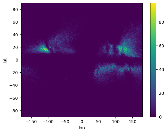
[8]:
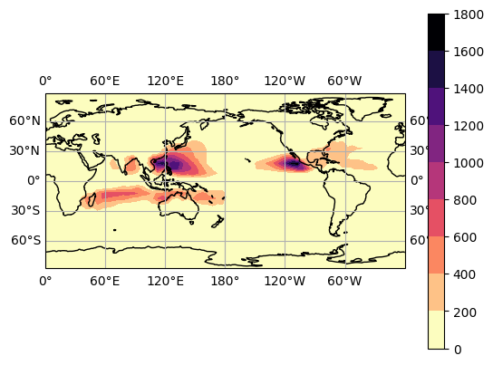
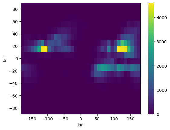
# Setting a larger bin_size
D = huracanpy.calc.density(tracks.lon, tracks.lat, bin_size=10)
D.plot()
D
/home/docs/checkouts/readthedocs.org/user_builds/huracanpy/envs/stable/lib/python3.12/site-packages/huracanpy/calc/_density.py:88: UserWarning: By default density does not take into account the spherical geometry ofthe Earth. Set spherical=True to account for this
  warnings.warn(
[8]:
<xarray.DataArray (lat: 18, lon: 36)> Size: 5kB
array([[0.000e+00, 0.000e+00, 0.000e+00, 0.000e+00, 0.000e+00, 0.000e+00,
        0.000e+00, 0.000e+00, 0.000e+00, 0.000e+00, 0.000e+00, 0.000e+00,
        0.000e+00, 0.000e+00, 0.000e+00, 0.000e+00, 0.000e+00, 0.000e+00,
        0.000e+00, 0.000e+00, 0.000e+00, 0.000e+00, 0.000e+00, 0.000e+00,
        0.000e+00, 0.000e+00, 0.000e+00, 0.000e+00, 0.000e+00, 0.000e+00,
        0.000e+00, 0.000e+00, 0.000e+00, 0.000e+00, 0.000e+00, 0.000e+00],
       [0.000e+00, 0.000e+00, 0.000e+00, 0.000e+00, 0.000e+00, 0.000e+00,
        0.000e+00, 0.000e+00, 0.000e+00, 0.000e+00, 0.000e+00, 0.000e+00,
        0.000e+00, 0.000e+00, 0.000e+00, 0.000e+00, 0.000e+00, 0.000e+00,
        0.000e+00, 0.000e+00, 0.000e+00, 0.000e+00, 0.000e+00, 0.000e+00,
        0.000e+00, 0.000e+00, 0.000e+00, 0.000e+00, 0.000e+00, 0.000e+00,
        0.000e+00, 0.000e+00, 0.000e+00, 0.000e+00, 0.000e+00, 0.000e+00],
       [0.000e+00, 0.000e+00, 0.000e+00, 0.000e+00, 0.000e+00, 1.000e+00,
        1.000e+00, 0.000e+00, 0.000e+00, 0.000e+00, 0.000e+00, 0.000e+00,
        0.000e+00, 0.000e+00, 0.000e+00, 0.000e+00, 0.000e+00, 0.000e+00,
        0.000e+00, 0.000e+00, 0.000e+00, 0.000e+00, 0.000e+00, 0.000e+00,
        0.000e+00, 0.000e+00, 0.000e+00, 0.000e+00, 0.000e+00, 0.000e+00,
        0.000e+00, 0.000e+00, 0.000e+00, 0.000e+00, 1.000e+00, 4.000e+00],
       [0.000e+00, 3.000e+00, 2.000e+00, 4.000e+00, 5.000e+00, 2.000e+00,
        2.000e+00, 0.000e+00, 0.000e+00, 0.000e+00, 0.000e+00, 0.000e+00,
...
        0.000e+00, 0.000e+00, 0.000e+00, 0.000e+00, 0.000e+00, 3.000e+00,
        1.600e+01, 3.300e+01, 1.610e+02, 1.180e+02, 1.910e+02, 2.610e+02],
       [0.000e+00, 0.000e+00, 0.000e+00, 0.000e+00, 1.000e+00, 0.000e+00,
        0.000e+00, 0.000e+00, 0.000e+00, 0.000e+00, 0.000e+00, 0.000e+00,
        1.700e+01, 2.000e+00, 9.000e+00, 2.400e+01, 2.800e+01, 1.500e+01,
        6.000e+00, 3.000e+00, 0.000e+00, 0.000e+00, 0.000e+00, 0.000e+00,
        0.000e+00, 0.000e+00, 0.000e+00, 0.000e+00, 0.000e+00, 0.000e+00,
        0.000e+00, 1.000e+00, 1.000e+01, 2.000e+00, 4.000e+00, 9.000e+00],
       [0.000e+00, 0.000e+00, 0.000e+00, 0.000e+00, 0.000e+00, 0.000e+00,
        0.000e+00, 0.000e+00, 0.000e+00, 0.000e+00, 0.000e+00, 0.000e+00,
        0.000e+00, 0.000e+00, 0.000e+00, 0.000e+00, 0.000e+00, 1.000e+00,
        0.000e+00, 0.000e+00, 0.000e+00, 0.000e+00, 0.000e+00, 0.000e+00,
        0.000e+00, 0.000e+00, 0.000e+00, 0.000e+00, 0.000e+00, 0.000e+00,
        0.000e+00, 0.000e+00, 0.000e+00, 0.000e+00, 0.000e+00, 0.000e+00],
       [0.000e+00, 0.000e+00, 0.000e+00, 0.000e+00, 0.000e+00, 0.000e+00,
        0.000e+00, 0.000e+00, 0.000e+00, 0.000e+00, 0.000e+00, 0.000e+00,
        0.000e+00, 0.000e+00, 0.000e+00, 0.000e+00, 0.000e+00, 0.000e+00,
        0.000e+00, 0.000e+00, 0.000e+00, 0.000e+00, 0.000e+00, 0.000e+00,
        0.000e+00, 0.000e+00, 0.000e+00, 0.000e+00, 0.000e+00, 0.000e+00,
        0.000e+00, 0.000e+00, 0.000e+00, 0.000e+00, 0.000e+00, 0.000e+00]])
Coordinates:
  * lat      (lat) float64 144B -85.0 -75.0 -65.0 -55.0 ... 55.0 65.0 75.0 85.0
  * lon      (lon) float64 288B -175.0 -165.0 -155.0 ... 155.0 165.0 175.0
Plotting#
[9]:
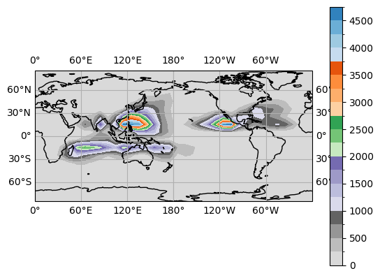
# With huracanpy's function
## The function is based on matplotlib's contourf, so you can use its options
huracanpy.plot.density(D, contourf_kws=dict(cmap="tab20c_r", levels=20))
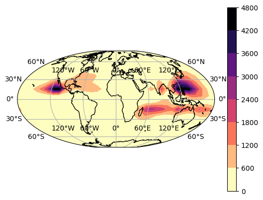
## Changing the projection with subplot_kws
huracanpy.plot.density(D, subplot_kws=dict(projection=ccrs.Mollweide()))
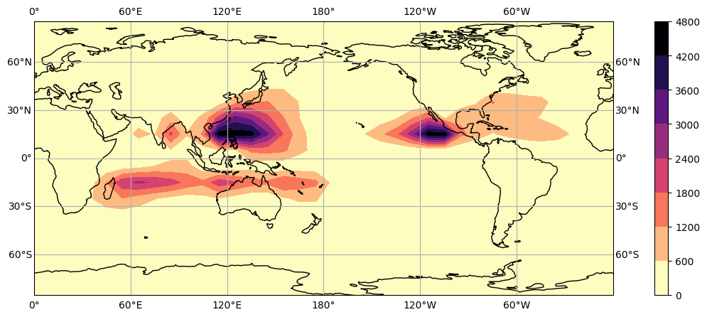
## Changing the figure's properties
huracanpy.plot.density(D, fig_kws=dict(figsize=(15, 5)))
[9]:
(<Figure size 1500x500 with 2 Axes>, <GeoAxes: xlabel='lon', ylabel='lat'>)