Basic use for assessing storm climatology in a dataset#
Here, we examplify usage of huracanpy with the dataset of TC in ERA-20C detected by the TRACK algorithm. This is meant to show an example of workflow. Please refer to specific parts of the documentation to learn about each part (e.g. loading, plotting, etc.) in more detail.
[1]:
import huracanpy

import matplotlib.pyplot as plt
import seaborn as sns
Read the file#
huracanpy’s load function can handle different track file types. Here, the data is available as a netcdf file.
[2]:
data = huracanpy.load(huracanpy.example_ERA20C_file)
data.psl.attrs["units"] = "hPa"  # Fixing misspelled pressure unit
data
/home/docs/checkouts/readthedocs.org/user_builds/huracanpy/envs/v1.4.0/lib/python3.12/site-packages/tqdm/auto.py:21: TqdmWarning: IProgress not found. Please update jupyter and ipywidgets. See https://ipywidgets.readthedocs.io/en/stable/user_install.html
  from .autonotebook import tqdm as notebook_tqdm
[2]:
<xarray.Dataset> Size: 2MB
Dimensions:         (record: 24865)
Coordinates:
    time            (record) datetime64[ns] 199kB ...
Dimensions without coordinates: record
Data variables:
    longitude_psl   (record) float32 99kB ...
    latitude_psl    (record) float32 99kB ...
    psl             (record) float64 199kB ...
    wind_speed_10m  (record) float32 99kB ...
    lon             (record) float32 99kB ...
    lat             (record) float32 99kB ...
    track_id        (record) <U7 696kB '1900-12' '1900-12' ... '2010-9' '2010-9'
Attributes:
    realm:        atmos
    history:      testing
    Conventions:  CF-1.7
featureType: trajectoryAdd useful information#
After loading, you can add various useful information for the analysis (basin, season, category…)
[3]:
# Use the accessor's add_ function to add the info you want
## SSHS category
data = data.hrcn.add_saffir_simpson_category(wind_name="wind_speed_10m")
## Presure category
data = data.hrcn.add_pressure_category(slp_name="psl")
## Season
data = data.hrcn.add_season()
# More info are available, in particular geographical ones, but we do not need them for
# this example.
[4]:
data
[4]:
<xarray.Dataset> Size: 2MB
Dimensions:                  (record: 24865)
Coordinates:
    time                     (record) datetime64[ns] 199kB 1900-07-23T18:00:0...
Dimensions without coordinates: record
Data variables:
    longitude_psl            (record) float32 99kB ...
    latitude_psl             (record) float32 99kB ...
    psl                      (record) float64 199kB 1.012e+03 ... 996.0
    wind_speed_10m           (record) float32 99kB 7.798 7.301 ... 12.17 19.06
    lon                      (record) float32 99kB ...
    lat                      (record) float32 99kB 9.978 10.07 ... 61.93 62.89
    track_id                 (record) <U7 696kB '1900-12' '1900-12' ... '2010-9'
    saffir_simpson_category  (record) int64 199kB -1 -1 -1 -1 -1 ... -1 -1 -1 0
    pressure_category        (record) int64 199kB -1 -1 -1 -1 -1 ... 0 0 0 0 0
    season                   (record) float64 199kB 1.9e+03 1.9e+03 ... 2.01e+03
Attributes:
    realm:        atmos
    history:      testing
    Conventions:  CF-1.7
featureType: trajectoryCheck the content of the file#
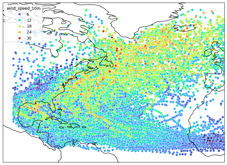
huracanpy provide a coarse plotting function that you can use for checking what is in your data.
[5]:
# Basic plot of the data points
data.hrcn.plot_tracks(intensity_var_name="wind_speed_10m")
[5]:
(<Figure size 1000x1000 with 1 Axes>, <GeoAxes: xlabel='lon', ylabel='lat'>)
/home/docs/checkouts/readthedocs.org/user_builds/huracanpy/envs/v1.4.0/lib/python3.12/site-packages/cartopy/io/__init__.py:242: DownloadWarning: Downloading: https://naturalearth.s3.amazonaws.com/110m_physical/ne_110m_coastline.zip
  warnings.warn(f'Downloading: {url}', DownloadWarning)
Climatological metrics#
You can compute basic statistics: frequency, TC days, ACE. Here shown as yearly averages.
[6]:
# Frequency (Number of track per year)
data.track_id.hrcn.nunique() / data.season.hrcn.nunique()
# number of unique tracks / number of unique season
[6]:
5.611111111111111
[7]:
# TCD (Accumulated duration of storms per year)
data.hrcn.get_track_duration().sum() / 24 / data.season.hrcn.nunique()
# Compute duration per track, convert to days / number of unique season
[7]:
<xarray.DataArray 'duration' ()> Size: 8B
array(56.71990741)
Attributes:
    standard_name:  time
    long_name:      Time
    time_calendar:   gregorian
    start:          1979010100
    step:           6
units: hours[8]:
# ACE per year
data = data.hrcn.add_ace(wind_name="wind_speed_10m")
data.ace.groupby(data.season).sum().mean()
# Get ace for each point, sum by season and average over the seasons
# NB: By default, huracanpy computes ACE only for points with wind above 34 knots
[8]:
<xarray.DataArray 'ace' ()> Size: 4B
array(5.252404, dtype=float32)
Attributes: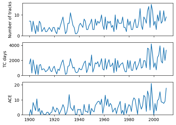
units: knot ** 2Variability#
With xarray’s grouping functionnalities, you can show variations of these statistics.
[9]:
## Interannual

fig, axs = plt.subplots(3, sharex=True)
# Frequency
# In this case, it is easier to go through a dataframe
data.to_dataframe().groupby("season").track_id.nunique().plot(ax=axs[0])
axs[0].set_ylabel("Number of tracks")
# TCD
data.groupby("season").apply(lambda s: s.hrcn.get_track_duration().sum()).plot(
    ax=axs[1]
)
axs[1].set_ylabel("TC days")
# ACE
data.groupby("season").sum().ace.plot(ax=axs[2])
axs[2].set_ylabel("ACE")

for ax in axs:
    ax.set_ylim(0)
    ax.set_xlabel("")
/home/docs/checkouts/readthedocs.org/user_builds/huracanpy/envs/v1.4.0/lib/python3.12/site-packages/xarray/structure/concat.py:674: UserWarning: No index created for dimension season because variable season is not a coordinate. To create an index for season, please first call `.set_coords('season')` on this object.
  ds.expand_dims(dim_name, create_index_for_new_dim=create_index_for_new_dim)
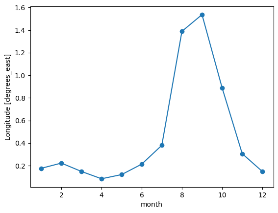
[10]:
## Seasonal

gen = data.hrcn.get_gen_vals()  # Extract the point of genesis for each track
(
    gen.groupby("time.month").count().lon  # compute number of genesis points per month
    / gen.season.hrcn.nunique()  # Normalize by number of season
).plot(marker="o")  # plot
[10]:
[<matplotlib.lines.Line2D at 0x7a947c7a2a50>]
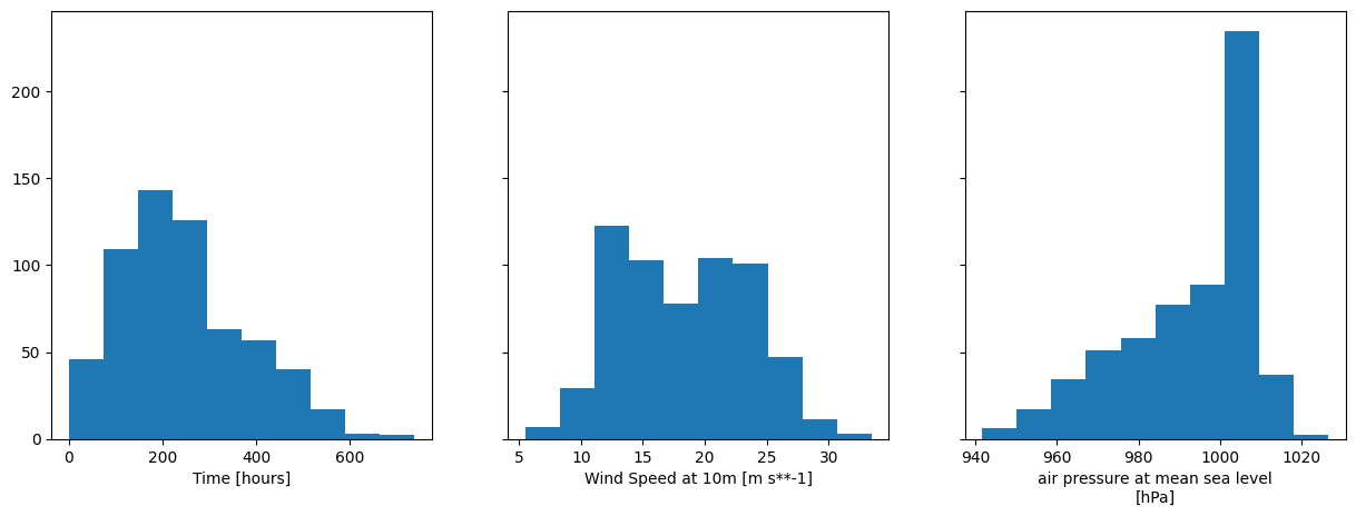
Track statistics#
You can also compute track-level statistics such as duration and lifetime maximum intensity.
[11]:
fig, axs = plt.subplots(1, 3, sharey=True, figsize=[15, 5])

# Duration
data.hrcn.get_track_duration().plot.hist(ax=axs[0])

# Maximum wind speed
data.wind_speed_10m.groupby(data.track_id).max().plot.hist(ax=axs[1])

# Minimum SLP
data.psl.groupby(data.track_id).min().plot.hist(ax=axs[2])
[11]:
(array([  6.,  17.,  34.,  51.,  58.,  77.,  89., 235.,  37.,   2.]),
 array([ 941.6126709 ,  950.1151001 ,  958.6175293 ,  967.1199585 ,
         975.6223877 ,  984.12481689,  992.62724609, 1001.12967529,
        1009.63210449, 1018.13453369, 1026.63696289]),
 <BarContainer object of 10 artists>)
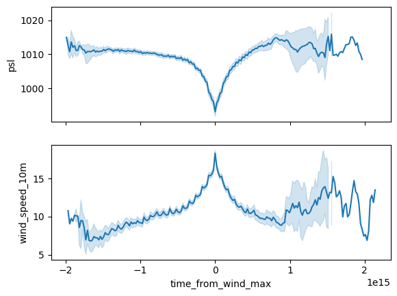
Lifecycles#
[12]:
# Compute times from extremum
data["time_from_slp_min"] = data.hrcn.get_time_from_apex(
    intensity_var_name="psl", stat="min"
)
data["time_from_wind_max"] = data.hrcn.get_time_from_apex(
    intensity_var_name="wind_speed_10m",
)
[13]:
# Plot with seaborn
fig, axs = plt.subplots(2, sharex=True)
# SLP lifecycle
sns.lineplot(data=data, x="time_from_slp_min", y="psl", ax=axs[0])
# Wind lifecycle
sns.lineplot(data=data, x="time_from_wind_max", y="wind_speed_10m", ax=axs[1])
[13]:
<Axes: xlabel='time_from_wind_max', ylabel='wind_speed_10m'>
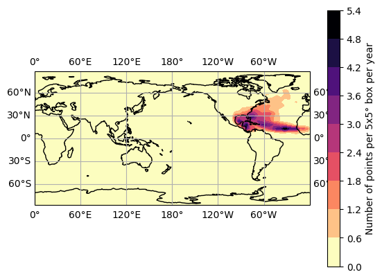
Track density#
[14]:
# Density of all points
d = data.hrcn.get_density(bin_size=5) / data.season.hrcn.nunique()
huracanpy.plot.density(
    d,
    cbar_kwargs=dict(label="Number of points per 5x5° box per year"),
)
/home/docs/checkouts/readthedocs.org/user_builds/huracanpy/envs/v1.4.0/lib/python3.12/site-packages/huracanpy/calc/_density.py:88: UserWarning: By default density does not take into account the spherical geometry ofthe Earth. Set spherical=True to account for this
  warnings.warn(
[14]:
(<Figure size 640x480 with 2 Axes>, <GeoAxes: xlabel='lon', ylabel='lat'>)
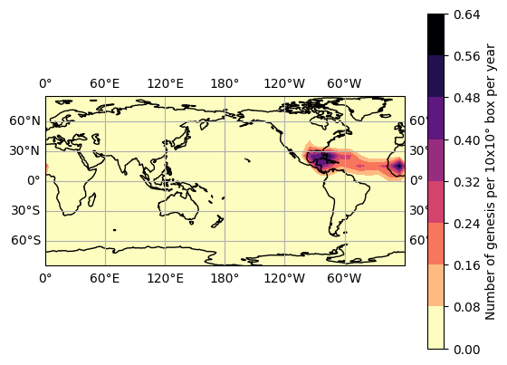
[15]:
# Density of all points
d = gen.hrcn.get_density(bin_size=10) / data.season.hrcn.nunique()
huracanpy.plot.density(
    d,
    cbar_kwargs=dict(label="Number of genesis per 10x10° box per year"),
)
/home/docs/checkouts/readthedocs.org/user_builds/huracanpy/envs/v1.4.0/lib/python3.12/site-packages/huracanpy/calc/_density.py:88: UserWarning: By default density does not take into account the spherical geometry ofthe Earth. Set spherical=True to account for this
  warnings.warn(
[15]:
(<Figure size 640x480 with 2 Axes>, <GeoAxes: xlabel='lon', ylabel='lat'>)